Usage

The swmmio.Model() class provides the basic endpoint for interfacing with SWMM models. To get started, save a SWMM5 model (.inp) in a directory with its report file (.rpt). A few examples:

import swmmio

# instantiate a swmmio model object
mymodel = swmmio.Model('/path/to/directory with swmm files')

# dataframe with useful data related to model nodes, conduits, and subcatchments
nodes = mymodel.nodes.dataframe
links = mymodel.links.dataframe
subs = mymodel.subcatchments.dataframe

# enjoy all the Pandas functions
nodes.head()

# write to a csv
nodes.to_csv('/path/mynodes.csv')

# calculate average and weighted average impervious
avg_imperviousness = subs.PercImperv.mean()
weighted_avg_imp = (subs.Area * subs.PercImperv).sum() / len(subs)

Nodes and Links Objects

Specific sections of data from the inp and rpt can be extracted with Nodes and Links objects. Although these are the same object-type of the swmmio.Model.nodes and swmmio.Model.links, accessing them directly allows for custom control over what sections of data are retrieved.

from swmmio import Model, Nodes
m = Model("coolest-model.inp")

# pass custom init arguments into the Nodes object instead of using default settings referenced by m.nodes() 
nodes = Nodes(
    model=m, 
    inp_sections=['junctions', 'storage', 'outfalls'],
    rpt_sections=['Node Depth Summary', 'Node Inflow Summary'],
    columns=[ 'InvertElev', 'MaxDepth', 'InitDepth', 'SurchargeDepth', 'MaxTotalInflow', 'coords']
)

# access data 
nodes.dataframe 

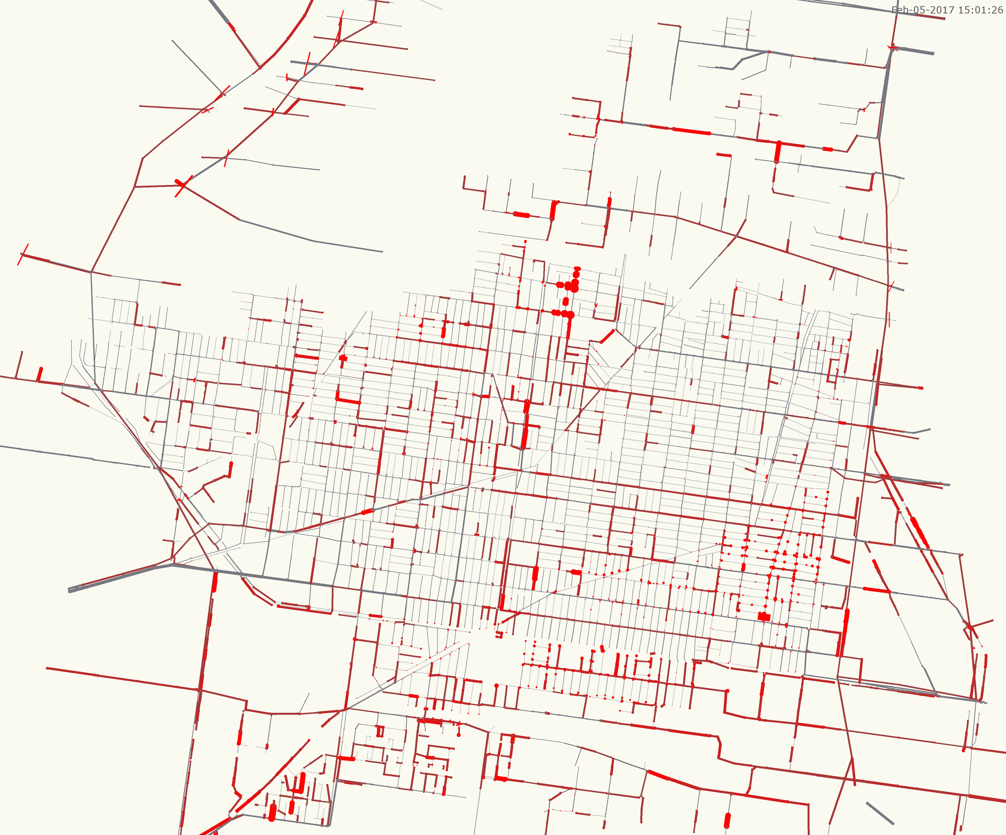
Generating Graphics

Create an image (.png) visualization of the model. By default, pipe stress and node flood duration is visualized if your model includes output data (a .rpt file should accompany the .inp).

swmmio.draw_model(mymodel)

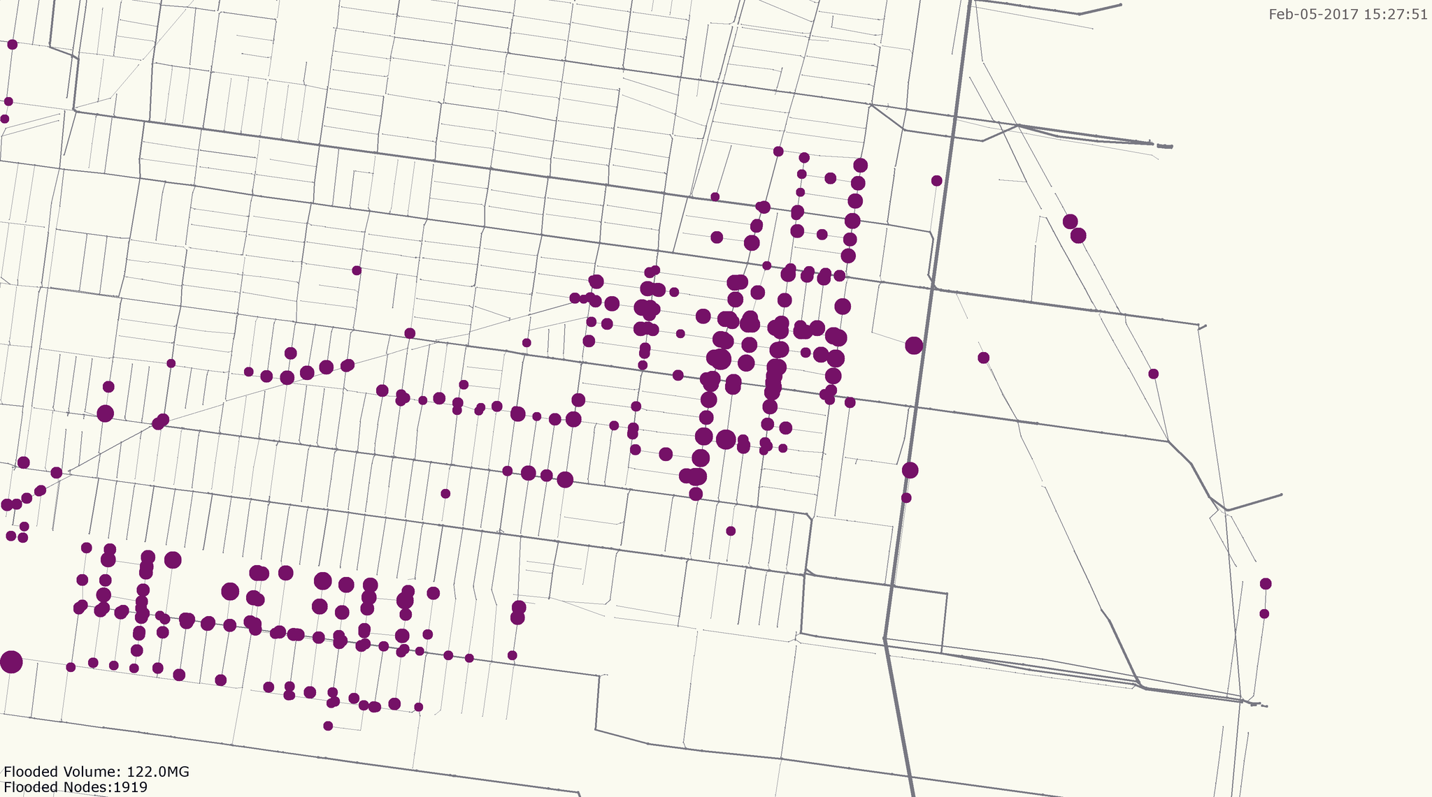
Use pandas to calculate some interesting stats, and generate a image to highlight what’s interesting or important for your project:

#isolate nodes that have flooded for more than 30 minutes
flooded_series = nodes.loc[nodes.HoursFlooded>0.5, 'TotalFloodVol']
flood_vol = sum(flooded_series) #total flood volume (million gallons)
flooded_count = len(flooded_series) #count of flooded nodes

#highlight these nodes in a graphic
nodes['draw_color'] = '#787882' #grey, default node color
nodes.loc[nodes.HoursFlooded>0.5, 'draw_color'] = '#751167' #purple, flooded nodes

#set the radius of flooded nodes as a function of HoursFlooded
nodes.loc[nodes.HoursFlooded>1, 'draw_size'] = nodes.loc[nodes.HoursFlooded>1, 'HoursFlooded'] * 12

#make the conduits grey, sized as function of their geometry
conds['draw_color'] = '#787882'
conds['draw_size'] = conds.Geom1

#add an informative annotation, and draw:
annotation = 'Flooded Volume: {}MG\nFlooded Nodes:{}'.format(round(flood_vol), flooded_count)
swmmio.draw_model(mymodel, annotation=annotation, file_path='flooded_anno_example.png')

Building Variations of Models

Starting with a base SWMM model, other models can be created by inserting altered data into a new inp file. Useful for sensitivity analysis or varying boundary conditions, models can be created using a fairly simple loop, leveraging the modify_model package.

For example, climate change impacts can be investigated by creating a set of models with varying outfall Fixed Stage elevations:

import os
import swmmio

# initialize a baseline model object
baseline = swmmio.Model(r'path\to\baseline.inp')
rise = 0.0 #set the starting sea level rise condition

# create models up to 5ft of sea level rise.
while rise <= 5:

    # create a dataframe of the model's outfalls
    outfalls = baseline.inp.outfalls

    # create the Pandas logic to access the StageOrTimeseries column of  FIXED outfalls
    slice_condition = outfalls.OutfallType == 'FIXED', 'StageOrTimeseries'

    # add the current rise to the outfalls' stage elevation
    outfalls.loc[slice_condition] = pd.to_numeric(outfalls.loc[slice_condition]) + rise
    baseline.inp.outfalls = outfalls
    
    # copy the base model into a new directory    
    newdir = os.path.join(baseline.inp.dir, str(rise))
    os.mkdir(newdir)
    newfilepath = os.path.join(newdir, baseline.inp.name + "_" + str(rise) + '_SLR.inp')
    
    # Overwrite the OUTFALLS section of the new model with the adjusted data
    baseline.inp.save(newfilepath)

    # increase sea level rise for the next loop
    rise += 0.25

Access Model Network

The swmmio.Model class returns a Networkx MultiDiGraph representation of the model via that network parameter:

# access the model as a Networkx MutliDiGraph
G = model.network

# iterate through links
for u, v, key, data in model.network.edges(data=True, keys=True):

        print (key, data['Geom1'])
        # do stuff with the network

Running Models

Using the command line tool, individual SWMM5 models can be run by invoking the swmmio module in your shell as such:

python -m swmmio --run path/to/mymodel.inp

If you have many models to run and would like to take advantage of your machine’s cores, you can start a pool of simulations with the --start_pool (or -sp) command. After pointing -sp to one or more directories, swmmio will search for SWMM .inp files and add all them to a multiprocessing pool. By default, -sp leaves 4 of your machine’s cores unused. This can be changed via the -cores_left argument.

# run all models in models in directories Model_Dir1 Model_Dir2
python -m swmmio -sp Model_Dir1 Model_Dir2  

# leave 1 core unused
python -m swmmio -sp Model_Dir1 Model_Dir2  -cores_left=1

Warning

Using all cores for simultaneous model runs can put your machine's CPU usage at 100% for extended periods of time. This probably puts stress on your hardware. Use at your own risk.